How the encoding works#
A deltacells tile stores the counts of about 10,000 cells in roughly 0.7 bytes per nonzero value, where an ordinary sparse matrix needs 8. This page explains how. The whole trick is one decision, storing the genes in order of decreasing total counts, followed by a few simple steps that take advantage of what that order does to the data.
The figures use a real shard of 10,000 cells and 38,046 genes, with about 4,500 detected genes per cell.
The data: two lists per cell#
A count matrix is mostly zeros, so it is stored in compressed sparse row (CSR) form. For each cell, CSR keeps only the genes that were detected, as two lists of the same length:
the gene indices, in increasing order, and
the counts of those genes.
In a plain CSR matrix each entry costs 8 bytes (a 4-byte index and a 4-byte count). To compress these two lists well, we want them to be made of small numbers that repeat a lot. The next steps arrange for that.
Step 1: sort the genes by decreasing total counts#
Add up each gene’s counts over many cells, and number the genes from the highest total to the lowest. A gene with a high total is detected in most cells, and a gene with a low total in only a few. After this renumbering, the genes that a cell detects are packed toward the start of its row.
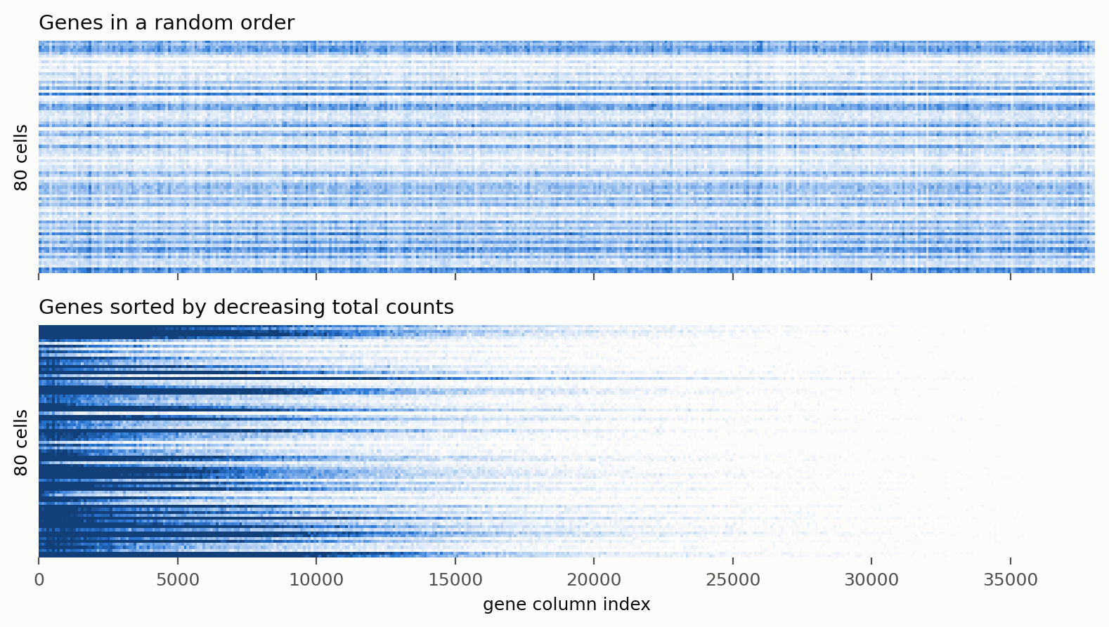
The genes detected in 80 cells (rows), with the genes in a random order (top) and sorted by decreasing total counts (bottom). Each pixel column is a bin of about 95 genes, and darker means that more of the bin’s genes were detected in that cell.#
In a random order, each cell’s detections are scattered over the whole row. Sorted, they form a dense block on the left that thins out to the right, and the same block shape repeats in every cell. That regularity is what the next steps use.
The converter computes this order once for the whole dataset, from the totals of up to 10 files spread evenly over the inputs,
and every tile uses it. The original gene of each stored column is kept (ds.gene_order), so the original order can always be
recovered.
Step 2: store the gaps between genes, not the genes#
Instead of the gene indices themselves, store the first index of each cell and then the gap from each detected gene to the next one (the “delta” coding of “deltacells”):
gene indices:  4   5   6   9  10  14  ...
stored gaps:   4   1   1   3   1   4  ...
Gene indices run up to tens of thousands, but gaps are small when the detected genes are close together, which is exactly what the sorted order produces.
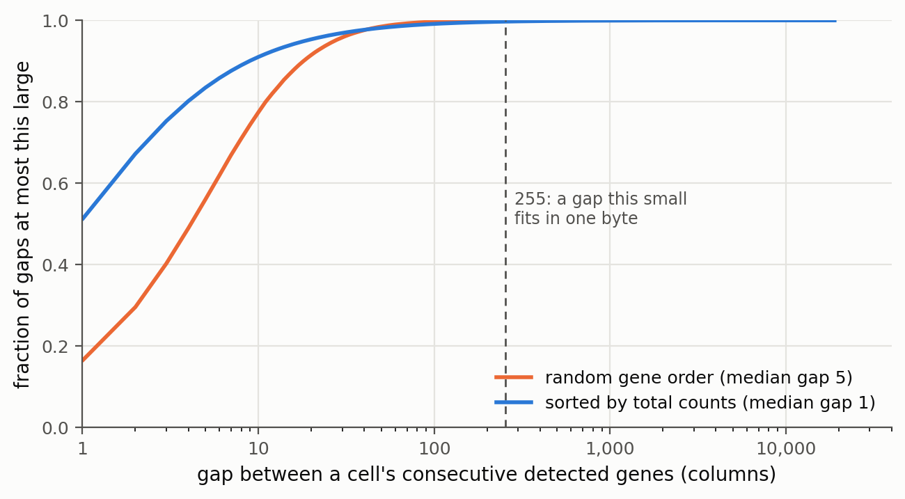
The distribution of the gaps between a cell’s consecutive detected genes, in the two orders. In the sorted order, 51% of the gaps are exactly 1 and the median gap is 1. In a random order, only 16% are 1 and the median is 5.#
In the sorted order, about three quarters of all gaps are 3 or less, and 99.7% fit in a single byte (255 or less). The gaps are not just small, they are repetitive: more than half are the same number. Repetition is what a compressor feeds on.
Step 3: the counts are small and repetitive too#
The counts of a single-cell experiment are mostly tiny. In this shard, half of the nonzero counts are exactly 1, 18% are 2, and 78% are 3 or less.
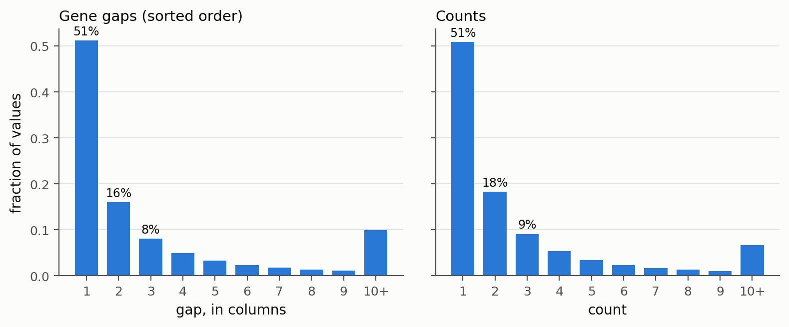
The two lists that are stored, as histograms of their values: the gaps in the sorted order (left) and the counts (right). The last bar in each chart groups all values of 10 or more.#
Zeros never appear in these lists. The sparse form already leaves them out, and the gaps account for them: a gap of 3 means “two zeros, then a detection”. Sorting pushes this further. Toward the right of a cell’s row, where the genes are rarely detected, what remains is a long run of detected genes with a count of 1 or 2, separated by small gaps. Here is a real stretch of one cell’s row, 24 consecutive detected genes:
gaps:    1, 3, 2, 1, 1, 1, 1, 1, 3, 3, 4, 2, 1, 1, 6, 1, 1, 4, 2, 8, 2, 3, 1, 2
counts:  1, 1, 1, 2, 1, 2, 1, 1, 1, 2, 1, 1, 1, 1, 1, 1, 3, 2, 1, 1, 6, 5, 1, 3
Both lists are made of a handful of small values that repeat. A 4-byte number for each of these is mostly wasted space.
Step 4: two lists of 16-bit integers#
Given that, the gaps and counts of a tile are each stored as an array of 16-bit unsigned integers (values up to 65,535), instead of 32-bit integers and floats.
Values that do not fit#
A few values are bigger than 65,535: a handful of very highly expressed genes, or, in a dataset with more than 65,536 genes, a gap between two detected genes that is wider than that. They are stored as the value 65,535 in the array, plus an entry in a small separate exception frame that holds the true value. Decoding reads the exceptions after the main arrays, so the common path does no extra work for them.
The exceptions must be rare. The writer refuses a tile with more than max(1024, nnz / 200) of them, because that is not what raw
counts look like.
Step 5: split into byte planes, then compress with zstd#
Each 16-bit array is split into its two bytes: all the low bytes first, then all the high bytes. For our two lists nearly all of the high bytes are 0, so the whole plane of high bytes compresses to almost nothing. The plane of low bytes holds the small repetitive numbers from the figures above.
Both planes then go through zstd, a general-purpose compressor. It finds repeated patterns and codes frequent byte values with fewer bits, which suits data that is a mix of a few common values (1, 2, 3, …) and rare larger ones. By default deltacells uses zstd level 19, a high level that gives small files, because the extra time is spent once when a dataset is written and does not slow down reading.
Step 6: independent chunks#
A tile is split into 8 chunks of about the same number of nonzeros, and each chunk is compressed separately. This costs about 0.5% in size or less. In exchange, the chunks can be encoded and decoded in parallel, one per thread, which is why decoding a tile takes 0.11 s on one core and 0.02 s on eight.
The result#
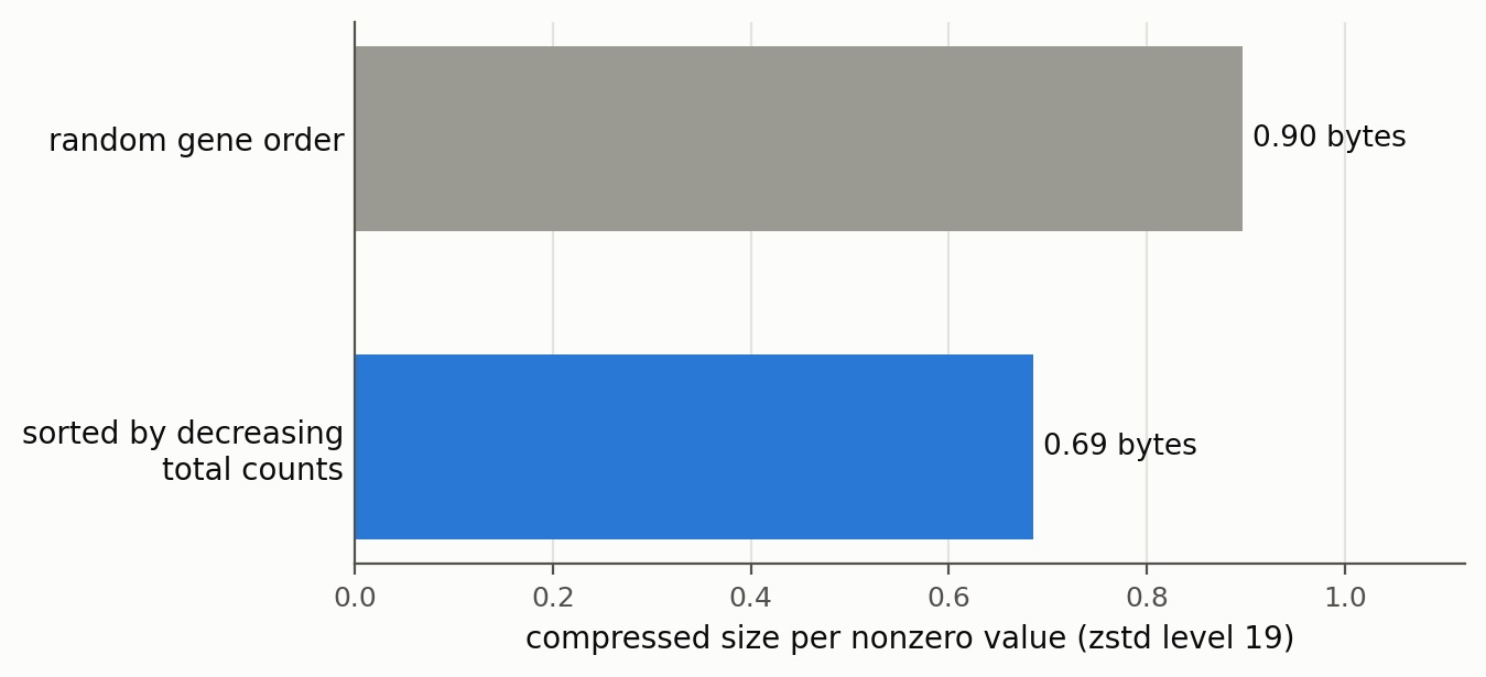
The compressed size of the same 10,000 cells, per nonzero value, with zstd level 19 and 8 chunks.#
With sorted genes, this shard takes 0.69 bytes per nonzero value. That is 24% smaller than the same data with its genes in a random order, and about 12 times smaller than the 8 bytes per value of an uncompressed CSR matrix. On a different real tile, measured on the benchmarks page, sorting saves 22% to 24% at every zstd level.
Why decoding is fast#
Decoding is the same steps in reverse, and every one of them is a simple pass over integers: decompress the chunks (in parallel), interleave the two byte planes back into 16-bit values, add up the gaps within each cell to recover the gene indices, and patch in the exceptions. The C core writes the result straight into the arrays of a CSR matrix, and it releases the Python GIL, so decoding several chunks or several tiles at once uses several cores. No AnnData or Arrow objects are created along the way.
Going further#
The format specification defines the exact byte layout of a tile and a dataset.
The benchmarks measure the size and the speed of every choice above: gene order, zstd level and number of chunks.
The figures on this page are made by
docs/make_figures.pyfrom a real shard of deeply-sequenced human neuronal snRNA-seq data from the BICAN consortium, and this data is harder to compress than random data from cellxgene. Compression gains from a random sample of cellxgene are larger.