Maximal Update Parametrization (μP) - coordinate checking
The purpose of this notebook is to illustrate the correctness of the MuLinear and Cerebras compatible μP implementations. This is done by calculating the average size of coordinates for a few training steps across the varying model widths for (a) pre-activation layers, (b) model weights, and (c) changes in model weights.
[1]:
import logging
import math
import warnings
from collections.abc import Callable
from typing import Any, Literal

import lightning.pytorch as pl
import matplotlib.pyplot as plt
import seaborn as sns
import torch
import torch.nn.functional as F
from torch import nn
from torchvision import datasets, transforms

from cellarium.ml.layers import MuLinear
from cellarium.ml.utilities.layers import create_initializer, scale_initializers_by_dimension
from cellarium.ml.utilities.mup import LRAdjustmentGroup
from cellarium.ml.utilities.testing import get_coord_data

logging.getLogger("lightning.pytorch").setLevel(logging.ERROR)
Data processing
The models are trained on CIFAR-10 dataset.
[2]:
data_dir = "/tmp"
batch_size = 64
transform = transforms.Compose([transforms.ToTensor(), transforms.Normalize((0.5, 0.5, 0.5), (0.5, 0.5, 0.5))])

trainset = datasets.CIFAR10(root=data_dir, train=True, download=True, transform=transform)
train_loader = torch.utils.data.DataLoader(trainset, batch_size=batch_size, shuffle=True)
Files already downloaded and verified
Model definitions
A simple 2-hidden-layer MLP with SP and muP. Notice that at base width Standard and μ Parametrizatons are identical. MLP with SP is given in [1].
[ ]:
# SP MLP
class MLP(pl.LightningModule):
    def __init__(
        self,
        width: int = 128,
        num_classes: int = 10,
        bias: bool = False,
        nonlin: Callable[[torch.Tensor], torch.Tensor] = F.relu,
        input_mult: float = 1.0,
        output_mult: float = 1.0,
        loss_fn: Callable[[torch.Tensor, torch.Tensor], torch.Tensor] = F.cross_entropy,
        optim_fn: type[torch.optim.Optimizer] = torch.optim.Adam,
        lr: float = 0.01,
        eps: float = 1e-8,
        weight_decay: float = 0.01,
    ) -> None:
        super().__init__()
        self.width = width
        self.bias = bias
        self.nonlin = nonlin
        self.input_mult = input_mult
        self.output_mult = output_mult
        self.loss_fn = loss_fn
        self.optim_fn = optim_fn
        self.lr = lr
        self.eps = eps
        self.weight_decay = weight_decay

        self.fc_1 = nn.Linear(3072, width, bias=bias)
        self.fc_2 = nn.Linear(width, width, bias=bias)
        self.fc_3 = nn.Linear(width, num_classes, bias=bias)
        self.reset_parameters()

    def reset_parameters(self) -> None:
        fan_in_1 = self.fc_1.weight.shape[1]
        nn.init.normal_(self.fc_1.weight, std=1 / math.sqrt(fan_in_1))  # 1 / sqrt(d)
        self.fc_1.weight.data /= self.input_mult
        fan_in_2 = self.fc_2.weight.shape[1]
        nn.init.normal_(self.fc_2.weight, std=1 / math.sqrt(fan_in_2))  # 1 / sqrt(n)
        nn.init.zeros_(self.fc_3.weight)  # zero readout
        if self.bias:
            # zero biases
            nn.init.zeros_(self.fc_1.bias)
            nn.init.zeros_(self.fc_2.bias)
            nn.init.zeros_(self.fc_3.bias)

    def forward(self, x: torch.Tensor) -> torch.Tensor:
        x = self.nonlin(self.fc_1(x) * self.input_mult)
        x = self.nonlin(self.fc_2(x))
        return self.fc_3(x) * self.output_mult

    def training_step(self, batch: tuple[torch.Tensor, torch.Tensor], batch_idx: int) -> torch.Tensor:
        data, target = batch
        output = self(data.view(data.size(0), -1))
        loss = self.loss_fn(output, target)
        return loss

    def configure_optimizers(self) -> torch.optim.Optimizer:
        optim_kwargs: dict[str, Any] = {"lr": self.lr}
        if self.optim_fn in [torch.optim.Adam, torch.optim.AdamW]:
            optim_kwargs["eps"] = self.eps
        if self.optim_fn == torch.optim.AdamW:
            optim_kwargs["weight_decay"] = self.weight_decay
        return self.optim_fn(self.parameters(), **optim_kwargs)


# muP MLP (MuLinear backend)
# Note: MuLinear layer automatically handles the scaling of the weights and learning rates
# The learning rate for individual layers are adjusted via internal parameter multipliers
# Gradients for Adam and AdamW are scaled via the hook in the parameters
class MuLinearMLP(pl.LightningModule):
    def __init__(
        self,
        width: int = 128,
        num_classes: int = 10,
        bias: bool = False,
        nonlin: Callable[[torch.Tensor], torch.Tensor] = F.relu,
        optimizer: Literal["sgd", "adam", "adamw"] = "sgd",
        input_mult: float = 1.0,
        output_mult: float = 1.0,
        loss_fn: Callable[[torch.Tensor, torch.Tensor], torch.Tensor] = F.cross_entropy,
        optim_fn: type[torch.optim.Optimizer] = torch.optim.Adam,
        lr: float = 0.01,
        eps: float = 1e-8,
        weight_decay: float = 0.01,
    ) -> None:
        super().__init__()
        self.width = width
        self.bias = bias
        self.nonlin = nonlin
        self.input_mult = input_mult
        self.output_mult = output_mult
        self.loss_fn = loss_fn
        self.optim_fn = optim_fn
        self.lr = lr
        self.eps = eps
        self.weight_decay = weight_decay

        self.fc_1 = MuLinear(
            in_features=3072,
            out_features=width,
            bias=bias,
            layer="input",
            optimizer=optimizer,
            weight_init_std=(1 / (math.sqrt(3072) * self.input_mult)),
            base_width=128,
        )
        self.fc_2 = MuLinear(
            in_features=width,
            out_features=width,
            bias=bias,
            layer="hidden",
            optimizer=optimizer,
            weight_init_std=(1 / math.sqrt(128)),
            base_width=128,
        )
        self.fc_3 = MuLinear(
            in_features=width,
            out_features=num_classes,
            bias=bias,
            layer="output",
            optimizer=optimizer,
            weight_init_std=0.0,
            base_width=128,
        )

    def forward(self, x: torch.Tensor) -> torch.Tensor:
        x = self.nonlin(self.fc_1(x) * self.input_mult)
        x = self.nonlin(self.fc_2(x))
        return self.fc_3(x) * self.output_mult

    def training_step(self, batch: tuple[torch.Tensor, torch.Tensor], batch_idx: int) -> torch.Tensor:
        data, target = batch
        output = self(data.view(data.size(0), -1))
        loss = self.loss_fn(output, target)
        return loss

    def configure_optimizers(self) -> torch.optim.Optimizer:
        optim_kwargs: dict[str, Any] = {"lr": self.lr}
        if self.optim_fn in [torch.optim.Adam, torch.optim.AdamW]:
            optim_kwargs["eps"] = self.eps
        if self.optim_fn == torch.optim.AdamW:
            optim_kwargs["weight_decay"] = self.weight_decay
        return self.optim_fn(self.parameters(), **optim_kwargs)


# muP MLP (Cerebras compatible)
# Note: This implementation explicitly handles the scaling of the weights and learning rates
# The learning rate for individual layers are adjusted via LRAdjustmentGroup
# Since the weight decay is coupled with the learning rate in AdamW, we need to decouple it
# by scaling it inversely with the learning rate.
# Also instead of scaling the gradients, here we scale down the eps for Adam and AdamW
class CerebrasMLP(pl.LightningModule):
    def __init__(
        self,
        width: int = 128,
        num_classes: int = 10,
        bias: bool = False,
        nonlin: Callable[[torch.Tensor], torch.Tensor] = F.relu,
        input_mult: float = 1.0,
        output_mult: float = 1.0,
        loss_fn: Callable[[torch.Tensor, torch.Tensor], torch.Tensor] = F.cross_entropy,
        optim_fn: type[torch.optim.Optimizer] = torch.optim.Adam,
        lr: float = 0.01,
        eps: float = 1e-8,
        weight_decay: float = 0.01,
    ) -> None:
        super().__init__()
        self.width = width
        self.bias = bias
        self.nonlin = nonlin
        self.input_mult = input_mult
        self.output_mult = output_mult
        self.loss_fn = loss_fn
        self.optim_fn = optim_fn
        self.lr = lr
        self.eps = eps
        self.weight_decay = weight_decay

        self.fc_1 = nn.Linear(3072, width, bias=bias)
        self.fc_2 = nn.Linear(width, width, bias=bias)
        self.fc_3 = nn.Linear(width, num_classes, bias=bias)
        self.fc_1_initializer = {"name": "normal_", "mean": 0.0, "std": 1 / (math.sqrt(3072) * self.input_mult)}
        self.fc_2_initializer = {"name": "normal_", "mean": 0.0, "std": 1 / math.sqrt(128)}
        self.fc_3_initializer = {"name": "zeros_"}
        width_mult = width / 128
        scale_initializers_by_dimension(
            self.fc_2_initializer,
            width_scale=width_mult**-0.5,
        )
        self.output_mult /= width_mult
        self.width_mult = width_mult
        self.lr_adjustment_groups = {"fc_2": LRAdjustmentGroup("*fc_2*weight")}
        self.lr_adjustment_groups["fc_2"].set_scale(1 / width_mult)
        self.reset_parameters()

    def reset_parameters(self) -> None:
        create_initializer(self.fc_1_initializer)(self.fc_1.weight)
        create_initializer(self.fc_2_initializer)(self.fc_2.weight)
        create_initializer(self.fc_3_initializer)(self.fc_3.weight)
        if self.bias:
            # zero biases
            nn.init.zeros_(self.fc_1.bias)
            nn.init.zeros_(self.fc_2.bias)
            nn.init.zeros_(self.fc_3.bias)

    def forward(self, x: torch.Tensor) -> torch.Tensor:
        x = self.nonlin(self.fc_1(x) * self.input_mult)
        x = self.nonlin(self.fc_2(x))
        return self.fc_3(x) * self.output_mult

    def training_step(self, batch: tuple[torch.Tensor, torch.Tensor], batch_idx: int) -> torch.Tensor:
        data, target = batch
        output = self(data.view(data.size(0), -1))
        loss = self.loss_fn(output, target)
        return loss

    def configure_optimizers(self) -> torch.optim.Optimizer:
        # Group parameters by learning rate adjustment group
        params_groups_dict: dict[str, list[torch.Tensor]] = {}
        for name, param in self.named_parameters():
            for lr_group_name, lr_group in self.lr_adjustment_groups.items():
                if lr_group.param_filter(name):
                    params_groups_dict.setdefault(lr_group_name, []).append(param)
                    break
            else:
                params_groups_dict.setdefault("default", []).append(param)

        # Create parameter groups for the optimizer
        param_groups = []
        for lr_group_name, params in params_groups_dict.items():
            group_optim_kwargs = {"lr": self.lr, "eps": self.eps / self.width_mult}
            if self.optim_fn == torch.optim.AdamW:
                group_optim_kwargs["weight_decay"] = self.weight_decay
            if lr_group_name != "default":
                group_optim_kwargs["lr"] *= self.lr_adjustment_groups[lr_group_name].scale
                if self.optim_fn == torch.optim.AdamW:
                    # weight_decay is coupled with the learning rate in AdamW
                    # so we need to decouple it by scaling it inversely with the learning rate
                    # see https://github.com/microsoft/mup/issues/1
                    group_optim_kwargs["weight_decay"] /= self.lr_adjustment_groups[lr_group_name].scale
            param_groups.append({"params": params, **group_optim_kwargs})

        return self.optim_fn(param_groups, **{})
Checking coordinate statistics
Following are the scaling rules for μP (Appendix J.2 of [1]):
Pre-activation layers (outputs): \(\Theta(1)\)
Input weights: \(W = \Theta(1)\) and \(\Delta W = \Theta(1)\)
Hidden weights: \(W = \Theta(1 / \sqrt{n})\) and \(\Delta W = \Theta(1 / n)\)
Output weights: \(W = \Theta(1 / n)\) and \(\Delta W = \Theta(1 / n)\)
All biases: \(b = \Theta(1)\) and \(\Delta b = \Theta(1)\)
[4]:
optim_dict = {"sgd": torch.optim.SGD, "adam": torch.optim.Adam, "adamw": torch.optim.AdamW}


# adapted from https://github.com/microsoft/mup/blob/main/examples/MLP/main.py
def coord_check_MLP(
    implementation: Literal["sp", "mup_mu_linear", "mup_cerebras"],
    bias: bool,
    nonlin: Callable[[torch.Tensor], torch.Tensor],
    lr: float,
    input_mult: float,
    output_mult: float,
    optim_name: Literal["adam", "adamw"],
    train_loader: torch.utils.data.DataLoader,
    nsteps: int,
    nseeds: int,
    widths: list[int],
) -> None:
    optim_fn = optim_dict[optim_name]

    def gen(w: int) -> Callable[[], pl.LightningModule]:
        def f() -> pl.LightningModule:
            model: pl.LightningModule
            if implementation == "sp":
                model = MLP(
                    width=w,
                    bias=bias,
                    nonlin=nonlin,
                    input_mult=input_mult,
                    output_mult=output_mult,
                    loss_fn=F.cross_entropy,
                    optim_fn=optim_fn,
                    lr=lr,
                )
            elif implementation == "mup_mu_linear":
                model = MuLinearMLP(
                    width=w,
                    bias=bias,
                    nonlin=nonlin,
                    optimizer=optim_name,
                    input_mult=input_mult,
                    output_mult=output_mult,
                    loss_fn=F.cross_entropy,
                    optim_fn=optim_fn,
                    lr=lr,
                )
            elif implementation == "mup_cerebras":
                model = CerebrasMLP(
                    width=w,
                    bias=bias,
                    nonlin=nonlin,
                    input_mult=input_mult,
                    output_mult=output_mult,
                    loss_fn=F.cross_entropy,
                    optim_fn=optim_fn,
                    lr=lr,
                )
            return model

        return f

    models = {w: gen(w) for w in widths}
    layer_name_to_multiplier_name = {"fc_1": "input_mult", "fc_3": "output_mult"}

    with warnings.catch_warnings():
        warnings.filterwarnings("ignore", message="The 'train_dataloader' does not have many workers")
        df = get_coord_data(
            models,
            layer_name_to_multiplier_name,
            train_loader,
            nseeds=nseeds,
            nsteps=nsteps,
        )

    # plot coordinates
    fig = plt.figure(figsize=(5 * nsteps, 10 + bias * 6))
    face_color = "xkcd:light grey" if implementation == "sp" else None
    if face_color is not None:
        fig.patch.set_facecolor(face_color)
    n_rows = 3 + bias * 2
    for t in range(nsteps):
        df_t = df[df.t == t]
        # outputs
        plt.subplot(n_rows, nsteps, t + 1)
        sns.lineplot(x="width", y="l1", data=df_t[(df_t.type == "out")], hue="module", legend=True if t == 0 else None)
        plt.title(f"t={t}")
        if t != 0:
            plt.ylabel("")
        plt.loglog(base=2, nonpositive="mask")

        # parameter values
        plt.subplot(n_rows, nsteps, t + 1 + nsteps)
        sns.lineplot(
            x="width",
            y="l1",
            data=df_t[(df_t.type == "param") & (df_t.module.str.contains("weight"))],
            hue="module",
            legend=True if t == 0 else None,
        )
        if t != 0:
            plt.ylabel("")
        plt.loglog(base=2, nonpositive="mask")

        # parameter deltas
        plt.subplot(n_rows, nsteps, t + 1 + nsteps * 2)
        sns.lineplot(
            x="width",
            y="l1",
            data=df_t[(df_t.type == "delta") & (df_t.module.str.contains("weight"))],
            hue="module",
            legend=True if t == 0 else None,
        )
        if t != 0:
            plt.ylabel("")
        plt.loglog(base=2, nonpositive="mask")

        if bias:
            # bias values
            plt.subplot(n_rows, nsteps, t + 1 + nsteps * 3)
            sns.lineplot(
                x="width",
                y="l1",
                data=df_t[(df_t.type == "param") & (df_t.module.str.contains("bias"))],
                hue="module",
                legend=True if t == 0 else None,
            )
            if t != 0:
                plt.ylabel("")
            plt.loglog(base=2, nonpositive="mask")

            # bias deltas
            plt.subplot(n_rows, nsteps, t + 1 + nsteps * 4)
            sns.lineplot(
                x="width",
                y="l1",
                data=df_t[(df_t.type == "delta") & (df_t.module.str.contains("bias"))],
                hue="module",
                legend=True if t == 0 else None,
            )
            if t != 0:
                plt.ylabel("")
            plt.loglog(base=2, nonpositive="mask")
    prm = "SP" if implementation == "sp" else "μP"
    suptitle = f"{prm} MLP {optim_name} lr={lr} nseeds={nseeds}"
    plt.suptitle(suptitle)
    plt.tight_layout(rect=[0, 0.03, 1, 0.95])
μP implementations differ for different optimizers, therefore, we have to check each optimizer separately.
Illustrating correctness of the μP implementation for the SGD optimizer
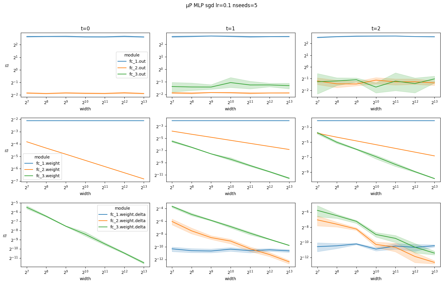
Notice how for the μP MLP coordinates scale with width according to the rules above at each time step. In particular, layer outputs are constant and do not explode with width.
[5]:
# optimal values for HPs at base width for SGD optimizer
# input_mult = 2**-4
# output_mult = 2**5
[6]:
# muP SGD (MuLinear)
coord_check_MLP(
    implementation="mup_mu_linear",
    bias=False,
    nonlin=F.relu,
    lr=0.1,
    input_mult=2**-4,
    output_mult=2**5,
    optim_name="sgd",
    train_loader=train_loader,
    nsteps=3,
    nseeds=5,
    widths=[2**i for i in range(7, 14)],
)
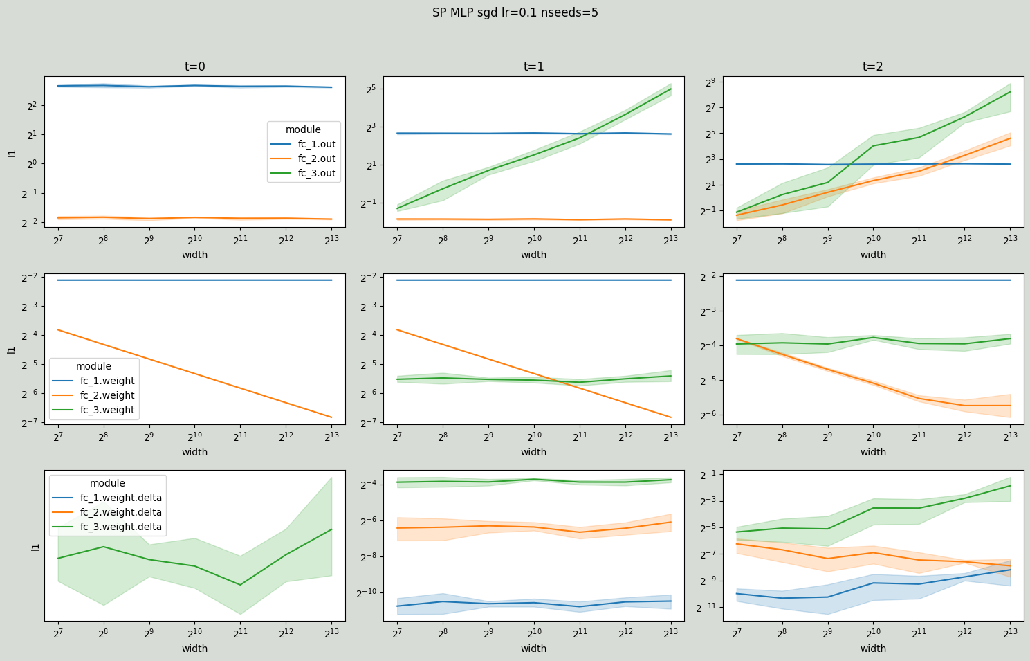
Now, notice how for SP MLP the layer outputs explode with width at time steps 1 and 2.
[7]:
# SP SGD
coord_check_MLP(
    implementation="sp",
    bias=False,
    nonlin=F.relu,
    lr=0.1,
    input_mult=2**-4,
    output_mult=2**5,
    optim_name="sgd",
    train_loader=train_loader,
    nsteps=3,
    nseeds=5,
    widths=[2**i for i in range(7, 14)],
)
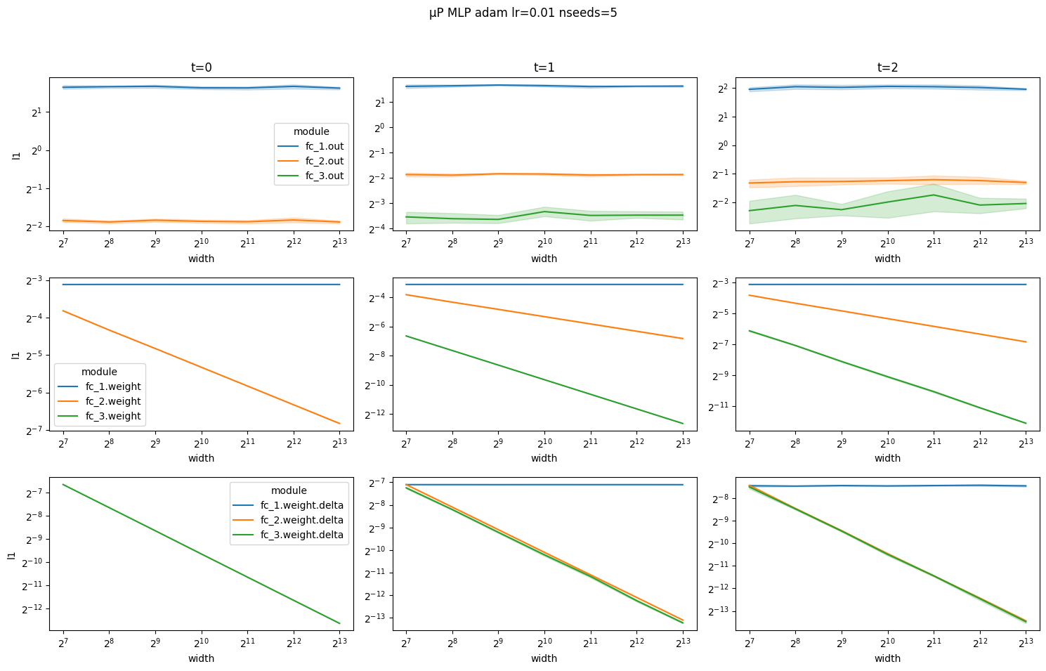
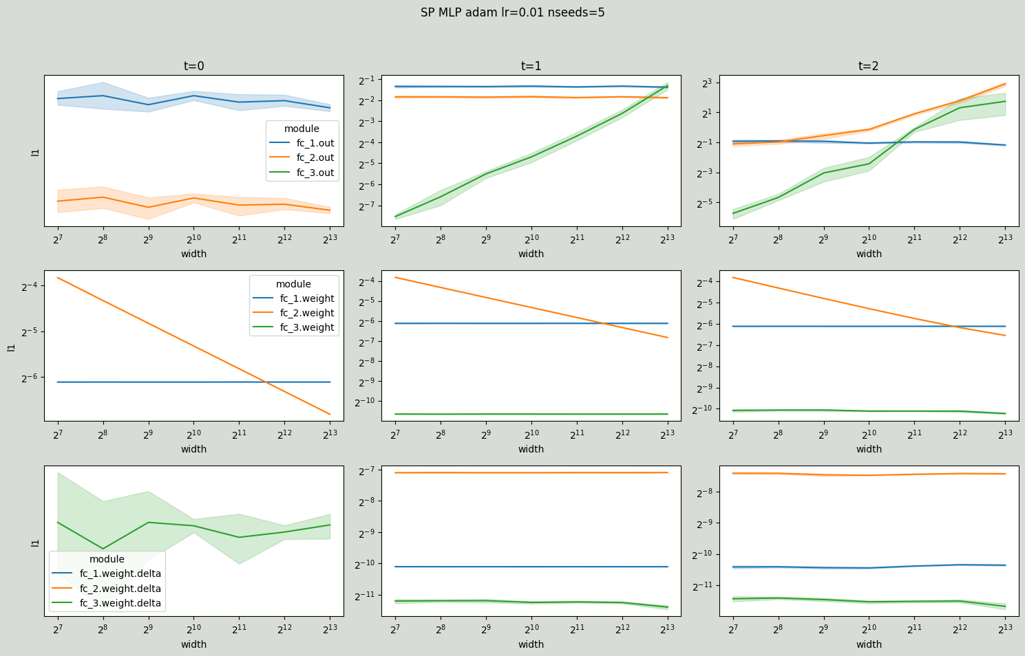
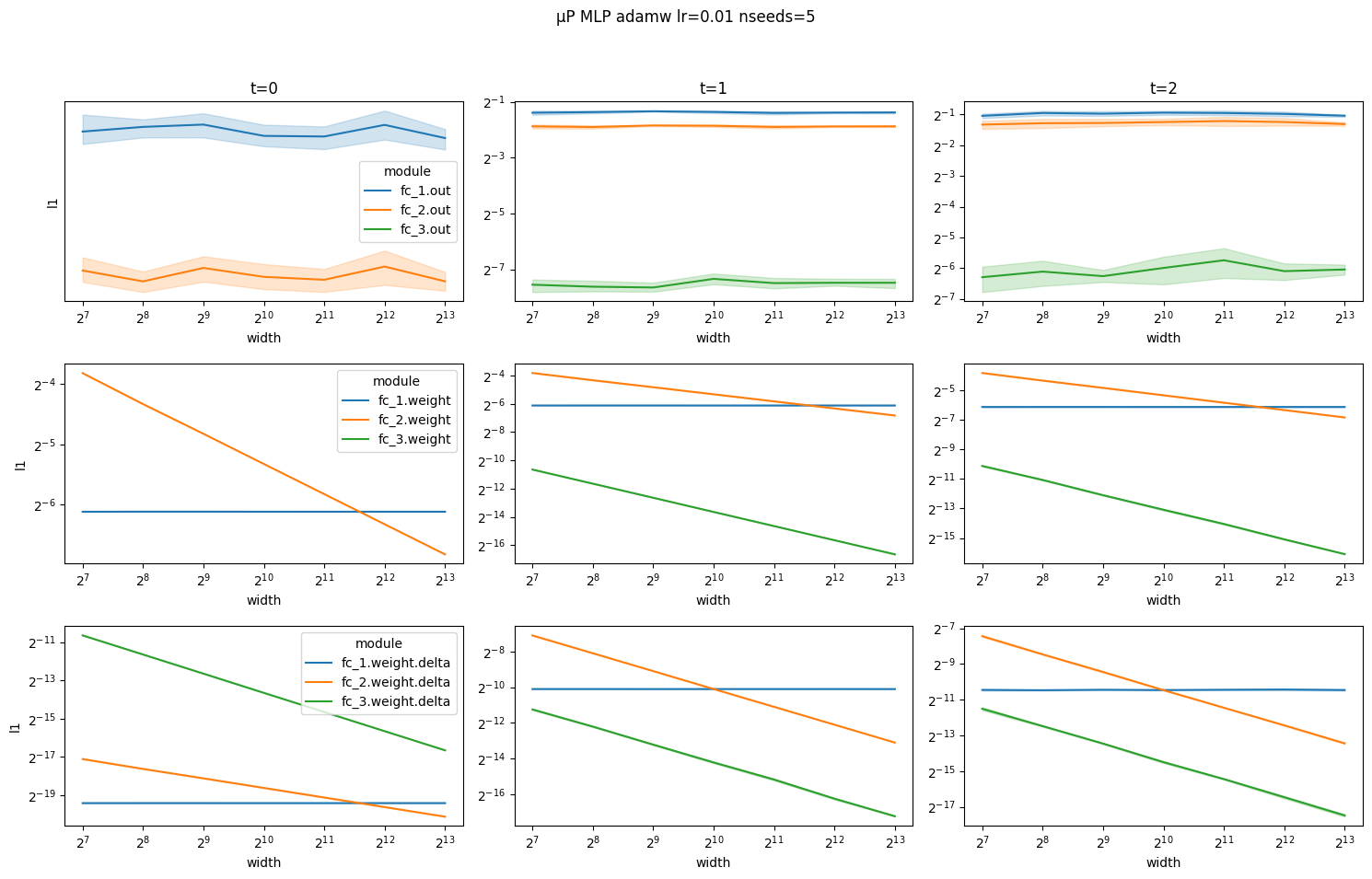
Illustrating correctness of the μP implementation for the Adam optimizer
Again, notice how coordinates scale according to the μP scaling rules.
[8]:
# optimal values for HPs at base width for Adam optimizer
# input_mult = 2**-3
# output_mult = 2**-4
[9]:
# muP Adam (MuLinear)
coord_check_MLP(
    implementation="mup_mu_linear",
    bias=False,
    nonlin=F.relu,
    lr=0.01,
    input_mult=2**-3,
    output_mult=2**-4,
    optim_name="adam",
    train_loader=train_loader,
    nsteps=3,
    nseeds=5,
    widths=[2**i for i in range(7, 14)],
)
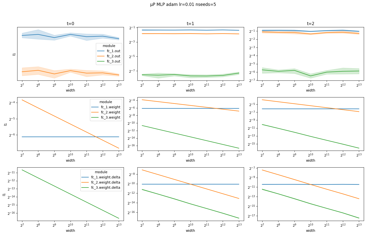
[10]:
# muP Adam (Cerebras compatible)
coord_check_MLP(
    implementation="mup_cerebras",
    bias=False,
    nonlin=F.relu,
    lr=0.01,
    input_mult=2**-3,
    output_mult=2**-4,
    optim_name="adam",
    train_loader=train_loader,
    nsteps=3,
    nseeds=5,
    widths=[2**i for i in range(7, 14)],
)
And layer outputs explode at time steps 1 and 2 for SP MLP.
[11]:
# SP Adam
coord_check_MLP(
    implementation="sp",
    bias=False,
    nonlin=F.relu,
    lr=0.01,
    input_mult=2**-3,
    output_mult=2**-4,
    optim_name="adam",
    train_loader=train_loader,
    nsteps=3,
    nseeds=5,
    widths=[2**i for i in range(7, 14)],
)
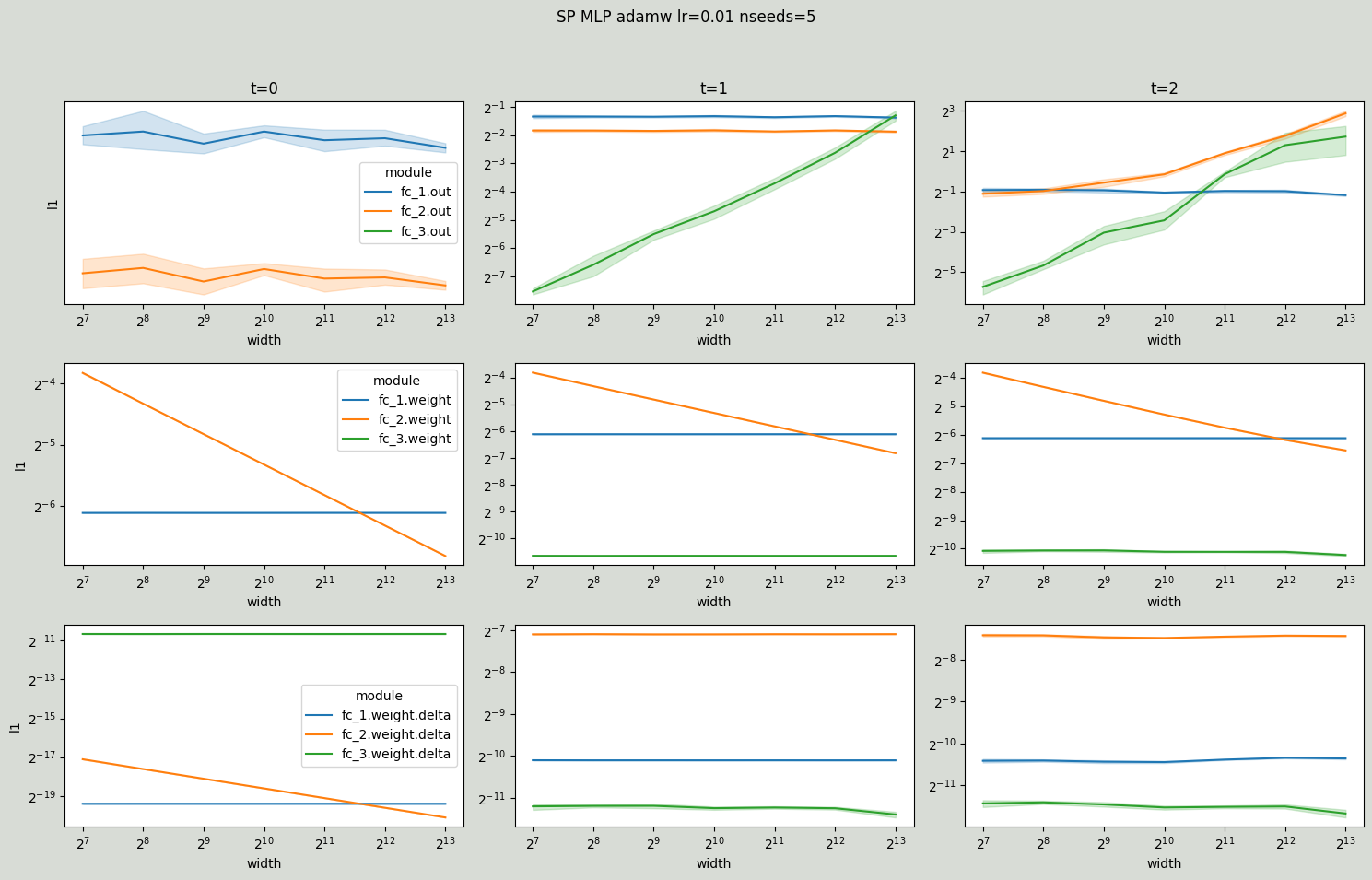
Illustrating correctness of the μP implementation for the AdamW optimizer
Same scaling rules apply for AdamW with one exception: for hidden layer weights ∆W is a combination of gradient updates Θ(1/n) and weight decay Θ(1/sqrt(n)) that scale differently. In particular, at time step 0 ∆W is only due to weight decay Θ(1/sqrt(n)) and at time steps 1 and 2 ∆W is dominated by the weight decay Θ(1/sqrt(n)).
[12]:
# muP AdamW (MuLinear)
coord_check_MLP(
    implementation="mup_mu_linear",
    bias=False,
    nonlin=F.relu,
    lr=0.01,
    input_mult=2**-3,
    output_mult=2**-4,
    optim_name="adamw",
    train_loader=train_loader,
    nsteps=3,
    nseeds=5,
    widths=[2**i for i in range(7, 14)],
)
[13]:
# muP AdamW (Cerebras compatible)
coord_check_MLP(
    implementation="mup_cerebras",
    bias=False,
    nonlin=F.relu,
    lr=0.01,
    input_mult=2**-3,
    output_mult=2**-4,
    optim_name="adamw",
    train_loader=train_loader,
    nsteps=3,
    nseeds=5,
    widths=[2**i for i in range(7, 14)],
)
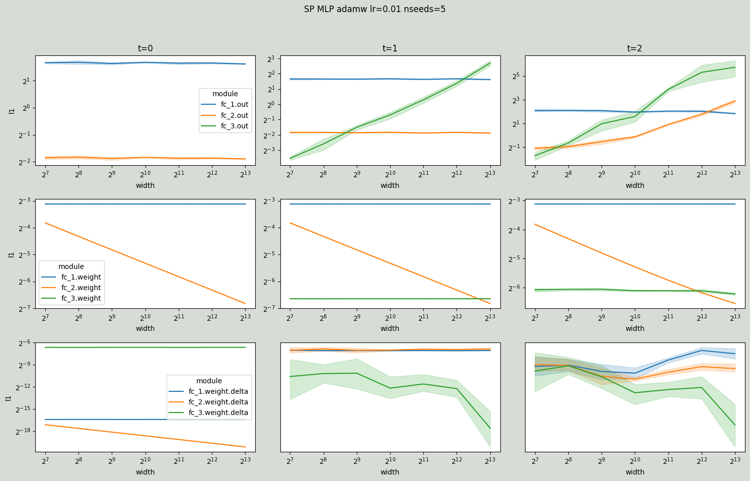
Again, for comparison SP MLP with exploding layer outputs.
[14]:
# SP AdamW
coord_check_MLP(
    implementation="sp",
    bias=False,
    nonlin=F.relu,
    lr=0.01,
    input_mult=2**-3,
    output_mult=2**-4,
    optim_name="adamw",
    train_loader=train_loader,
    nsteps=3,
    nseeds=5,
    widths=[2**i for i in range(7, 14)],
)
References: